With a Cobb-Douglas Production Function, the Differential Equation for the Solow Growth Model has a Closed-Form Solution—Tsering Sherpa and Miles Kimball

My “Ethics, Happiness and Choice” student (and research assistant) Tsering Sherpa did a project for her differential equation class on the Solow growth model. I was surprised to find out that the differential equation for the Solow Growth Model with a Cobb-Douglas production function has a closed-form solution. I proposed to Tsering that we coauthor a post on that. Here it is:
Economics put simply is the study of scarcity. The goal of economics is to study how resources are allocated, especially scarce resources. In order to do this, economists may use differential equations to model their analysis. A differential equation expresses the rate of change of the current state as a function of the current state, or in simpler terms, “an equation that involves an unknown function and its derivatives” (McOwen). More specifically, for the purposes of this post we look at ordinary differential equations. These are differential equations that only involve one independent variable. Ordinary differential equations relate to economics because they are the foundation for a multitude of mathematical concepts in economics. For example, the neoclassical growth theory introduced by Robert Solow and Trevor Swan in 1956 uses ordinary differential equations to describe how steady economic growth results from three main factors: labor, capital, and technology. This theory is also known as the Solow Growth Model.
The Solow Growth Model assumes capital and labor are being used efficiently, as well as that population growth, saving rate, and technology are constant. It also assumes a production function that is homogeneous of degree one: constant returns to scale. The goal is to solve for capital per worker, k, as a function of time. This shows exactly how capital per worker—and therefore the model economy—converges to its steady-state level, where the amount of capital lost by depreciation is offset by saving.
The differential equation driving the movements of capital per worker, k, is:

This equation gives the rate of change of capital per worker as a function of the fixed saving rate, s, the current level of capital per worker, k, output per worker, f(k), and the fixed depreciation rate, δ. The assumption of a Cobb-Douglas production function yields the more specific differential equation,

where 0< α < 1. The stipulation that 0< α represents capital being productive, while α < 1 represents the diminishing marginal returns to capital per worker. A is the rate of technological progress. The initial condition is

A change of variables reduces the differential equation (1) to a linear differential equation that can be solved by the usual integrating factor. Define

Then

The integrating factor is

Multiplying both sides by this integrating factor and rearranging:

Thus, using an indefinite integral:

where C is the constant of integration. The initial condition is:


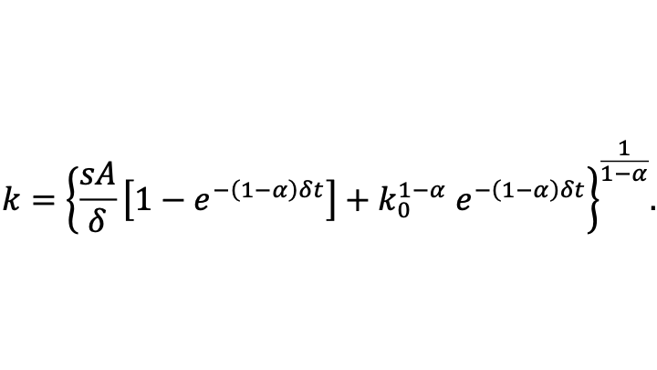
Thus,

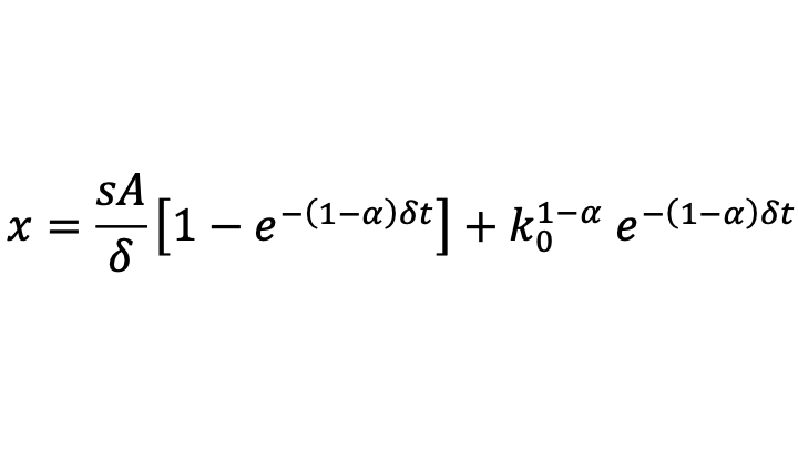
The steady-state value of capital per worker can then be seen as the limit of capital per worker as time goes to infinity:

The formula for capital per worker k is therefore a constant-elasticity-of-substitution (CES) aggregate between the initial level of capital per worker and the steady-state level of capital per worker k* given above, with elasticity of substitution equal to 1/α > 1 and a weight on the initial level of capital per worker that starts at 1 and exponentially decays at the rate (1-α)δ with the steady-state level of capital per worker k* having a complementary weight such that the two weights add to 1.
The formula for capital per worker, which drives all the other evolving variables in the model, implies that the convergence rate is equal to (1-α)δ. (That convergence rate generalize to cases with other production functions, as long as α is interpreted as capital’s share at the steady-state level of capital per worker.) This is a quite slow rate of convergence. For example, even if δ is relatively high, at a continuous-time rate of 10.5% per year, convergence would be a continuous-time rate of 7% per year if capital’s share is equal to 1/3. That means by the rule of 70 that the half-life of departures from the steady-state would be ten years, as the economy nears the steady state. (The rule of 70 is simply a consequence of the the natural logarithm of 2 equaling approximately .7.)
At the steady state, capital per worker is unchanging over time. That also means that unchanging at the steady state. Intuitively, investment is enough to compensate for depreciation. If there is population growth, or growth in the effective number of workers beyond population growth because of technological progress, the differential equation and its solution above continue to hold as long as k is interpreted as capital per effective worker and δ is interpreted as
δ = depreciation rate + population growth rate + rate of labor augmenting technological progress.
The power

is then the initial level of labor-augmenting technology, since labor-augmenting technology has to be taken to the power labor’s share (1-α) to be in multiplicative technology units, and conversely multiplicative technology level A has to be taken to the power of the reciprocal of labor’s share to be in labor-augmenting technology units. To see that, start with the two equivalent forms of the production function before the constant returns to scale has been used to express things in per effective worker terms. Here K is the overall level of capital, L is the overall number of workers and EL is the overall number of effective workers:

This equivalence implies

An interesting observation from the model is that two countries, regardless of the initial conditions for labor and capital, with the same savings, population growth, and depreciation rate will have the same steady state level of capital, thus both countries would conditionally converge (where the poor country grows faster along this convergence path).
Another important aspect of the Solow Growth Model is that interventions such as changing the saving rate will change the level of steady state per capita output, but will not permanently change the growth rate of per capita output.
In addition to its importance for economics, the Solow Growth Model provides a useful analogy for the effect of eating patterns on weight. As Miles discusses in “Kevin D. Hall and Juen Guo: Why it is So Hard to Lose Weight and So Hard to Keep it Off,” Permanent weight loss requires permanent changes in behavior, just as in the Solow Growth Model permanent changes in capital per effective worker require permanent changes in the saving rate.
Update, June 25, 2022, PM: Tweets from Dejanir Silva and Chris Edmond point out that Robert Solow himself showed this result and that this result was recapitulated by Chad Jones.
Update, June 29, 2022: Also see these tweets from Alex Zevelev for more growth models that can be solved in closed form.
References
Acemoglu, Daron. MIT Economics. 1 Nov. 2011, https://economics.mit.edu/files/7181.
Banton, Caroline. “The Neoclassical Growth Theory Explained.” Investopedia, Investope- dia, 19 May 2021, https://www.investopedia.com/terms/n/neoclassical-growth-theory.asp.
McOwen, Robert C. Worldwide Differential Equations with Linear Algebra. Worldwide Center of Mathematics, LLC, 2012.
“Solow Growth Model.” Corporate Finance Institute, 31 Jan. 2021, https://corporatefinanceinstitute.com/resources/knowledge/economics/solow-growth- model/.
Whelan, Karl. Topic 1: The Solow Model of Economic Growth. Trinity College Dublin, 2005, https://www.tcd.ie/Economics/staff/whelanka/topic1.pdf.