Sequencing of Projects, Continued
This post pushes the results in “Sequencing of Projects” further. To understand this post, you need to read “Sequencing of Projects” first. Here is a reminder of the notation:

The objective is to minimize total cost:
Total Cost = Cost of Completing Projects + Cost of Delay in Getting the Benefits from Completed Projects

One thing I leave undone in “Sequencing of Projects” is determining which project should be done first after accounting for the fact that later projects should be done more slowly, so that changing the order optimally means changing how slowly each project is done.
The first-order condition for the slowness of project i is:

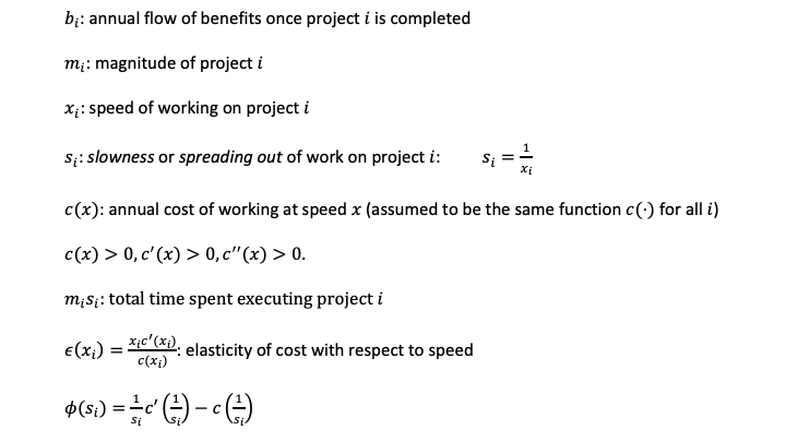
Diagrammatically:

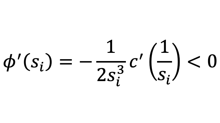
Both the downward slope and the convexity of phi(s_i) are important here. The downward slope follows from computing the first derivative of phi:
The second derivative of phi, which determines the curvature of phi, is:

Note the importance of the assumption that c’’’>0 for establishing the sign of phi’’. The assumption that c’’’(x_i)>0 is natural if one represents a maximum possible speed as cost going to infinity as that maximum possible speed is approached. A smooth function that goes up to infinity as it approaches a finite upper bound must have all positive derivatives as it approaches that upper bound.
Suppose some particular sequencing of projects has been proposed. Now consider switching the order of two consecutive projects in that proposed sequencing: A and B. Since this switch leaves unchanged the sequencing before these two projects, define b** as the sum of flow benefits from completing these two projects and all the projects sequenced after them and s** as the slowness optimal for that sum of flow benefits all waiting on completion of a project. Note that s** is, in fact, the optimal speed for whichever of projects A and B comes first between the two.
Let me determine which of [A, then B] or [B then A] with optimal slowness is better by looking at how much each improves on [A, then B] with the slowness of both A and B constrained to be s**.
As an intermediate good in making this calculation, I compute that the change in total cost from switching from [A, then B] with the slowness of both A and B constrained to be s** to [B, then A] with the slowness of both A and B constrained to be s** is

since switching to B, then A (with both at slowness s**) reduces the time to get to the benefit for B by how long project A takes, while the time to get to the benefit for A is increased by how long project B takes. Note that if the slownesses really were both constrained to be the same for both A and B, then the condition for A, then B being better would be:

or

But when the slownesses are freed up, there is another set of terms in comparing the total cost of [A, then B] to the total cost of [B, then A]. Adjusting the slowness of the second of the two projects to its optimum reduces total cost. That reduction in cost from slowing down the second project as compared to s** will be different depending on which project is second. The net reduction in total cost from slowing down a project is directly proportional to the magnitude of the project, because both the cost of completing the project and the cost of delay of things waiting on that project are proportional to the magnitude of the project. The other factor in the net reduction in total cost from slowing down a project can be shown geometrically as a triangle. The figures below show that triangle for both A and B. (I show the flow benefit from A as greater than the flow benefit of B.) Note that Triangle_A on the left is actually a function of b_B, while Triangle_B on the left is actually a function of b_A.

Including the adjustment of the slowness of the second project, the condition for switching from [A, then B] to [B, then A] to raise total costs is now:

Note that there is a shift to subtracting the magnitude of A times the Triangle for adjusting the pace of A instead of the corresponding product for B.
Using the fact that each Triangle is a function of the flow benefit of the other of the two projects, this is:

Rearranging:

Note that the curvature of phi guarantees that the function Triangle(b) grows faster than a quadratic in b. The message I get from this equation is that when the slowness is endogenized, a 1% change in the flow benefit b is more important in making a project more attractive to put first than is a 1% reduction in the magnitude m of the project. By contrast, if the slownesses were exogenously given, what would matter would be just the ratio b/m, which has a 1% increase in b and a 1% reduction in m equally important. So endogenizing the pace at which each project is done makes the benefit of each relatively more important in determining the best sequence.
Note that satisfying this condition for which of two consecutive projects should come first may not preclude reducing total cost be some other kind of rearrangement in the timing. That is one of the ways in which the problem if optimally sequencing projects is a difficult problem.